The section is a replication by work of McElreath (2020) who uses simulated data to explore how causal effects can be confounded through improper inclusion of control variables in statistical models. Here we will specifically focus on attempting to discern the treatment effect of a variable on an outcome variable but we will include un-observables as well as potential confounders. The author’s original video used for this replication can be seen at Statistical Rethinking video(s). We specifically explore the problem of including a Precision Parasite and how this actually turns into a Bias Amplifier if there are other omitted variables at play in the true model.
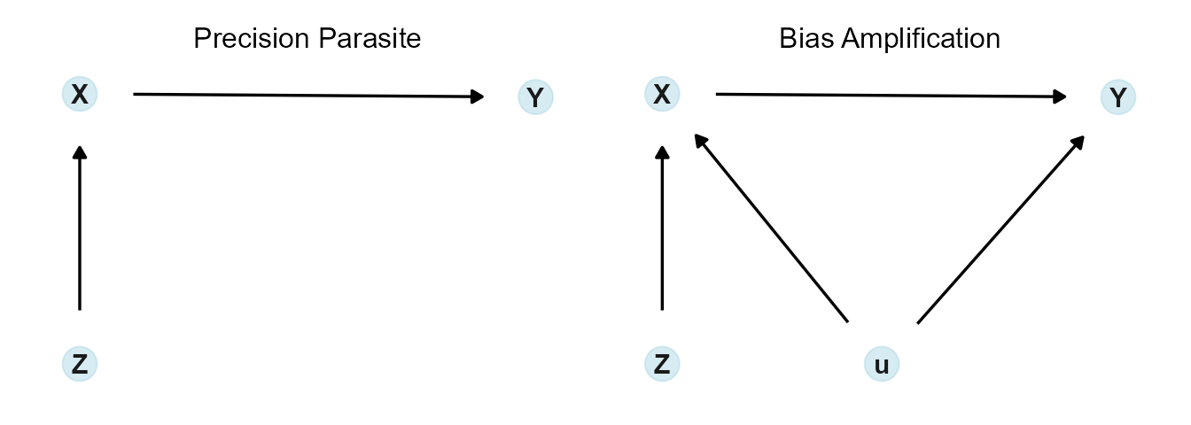
Simulation model for the “Precision Parasite” and the “Bias Amplifier”.
Show code
# Load required librarieslibrary("tidyverse")library("modelsummary")library("janitor")library("broom")library("glue")library("kableExtra")library("patchwork")library("ggdag")library("dagitty")# Adapted from @Kurz2023:gg_simple_dag <-function(d) { d %>%ggplot(aes(x = x, y = y, xend = xend, yend = yend)) +geom_dag_point(color ="lightblue", alpha =1/2, size =6.5) +geom_dag_text(color ="gray10") +geom_dag_edges() +theme_dag()}d_parasite <-dagitty("dag { bb=\"0,0,1,1\" X [exposure,pos=\"0.352,0.453\"] Y [outcome,pos=\"0.730,0.450\"] Z [pos=\"0.352,0.201\"] X -> Y Z -> X}")d_bias_amplification <-dagitty(" dag { bb=\"0,0,1,1\" X [exposure,pos=\"0.352,0.453\"] Y [outcome,pos=\"0.730,0.450\"] Z [pos=\"0.352,0.201\"] u [latent,pos=\"0.534,0.201\"] X -> Y Z -> X u -> X u -> Y }")p1 <-gg_simple_dag(d_parasite) +labs(subtitle ="Precision Parasite")p2 <-gg_simple_dag(d_bias_amplification) +labs(subtitle ="Bias Amplification")(p1 | p2) &theme(plot.subtitle =element_text(hjust =0.5))
Figure 3.1: Some Examples of Bad Controls (McElreath 2020)
These models in Figure 3.1 illustrate a few important concepts in statistical modelling. In the “Precision Parasite”\(z\) is not confounding the effect we are looking for of \(x\) on \(y\). Including \(z\) as a control variable seems harmless, however, the problem is that even though the estimated \(\beta\) coefficient on \(x\) remains unchanged when we include \(z\), the precision of \(\beta\) becomes worse. A more uncertain estimator could lead us to incorrectly fail to reject the null hypothesis that \(\beta = 0\) at some given statistical significance level.
The “Bias Amplification” situation shown in Figure 3.1 is an even more serious problem. Here we also have some un-observable variables that are acting as a fork for the effect of \(x\) on \(y\). We already know from basic econometrics that failing to capture these un-observables biases or confounds the estimate \(\beta\) on our variable of interest \(x\). Now, however, if we include \(z\) as a control variable, the bias actually increases.
To illustrate this, we will first produce a “Precision Parasite” and “Bias Amplification” examples with simulated data, then we will turn to the tried and true education data from Wooldridge (2019) and see if we can discover the same outcomes using real data. The following analysis is based on the following set of linear equations.
\(\alpha_1 = 1.5\): The constant term for log(Income).
\(\beta_1 = 0.1\): The effect of Education on log(Income).
\(\alpha_2 = 6.5\): The constant term for Education
\(\gamma_1 = 0.55\): The effect of Parents’ Education on Individual’s Education.
\(\epsilon\): Error terms for unobserved factors influencing Education and log(Income).
In this first set of equations the true model does not contain “Ability”. In other words, in Equation 3.1 and Equation 3.2, there are no variables confounding the model. Only the parent term \(Parent Education\) is acting through \(Education\) but has no direct influence on \(log(Income)\). The following set of linear equations explicitly shows the omitted variable \(Ability\).
Where all variables are the same as in the first specification, except: - \(\beta_2 = 0.3\): The effect of Ability on log(Income). and - \(\gamma_2 = 0.6\): The effect of Ability on Individual’s Education.
Note the error term is the same in both models. In the second model, the fork\(Ability\) will be omitted from the regression model for exploration of how inclusion of the “Precision Parasite” actually exacerbates the bias introduced from an omitted variable.
Table 3.1 shows summary statistics for the simulated data-set.
Show code
set.seed(1234)# Number of observationsn <-1000# Simulate an (un)observed confounder (ability) affecting educationability <-rnorm(n)# Simulate an observed value of parent's x (education) affecting x (education)parent_educ <-rnorm(n, mean =12)# Simulate x (education) influenced by z (parent's education)educ <-6.5+0.55* parent_educ +rnorm(n)educ_bias <-6.5+0.55* parent_educ +0.6* ability +rnorm(n)# Simulate income, influenced by x and Zlog_income <-1.5+0.1* educ +rnorm(n)# Simulate omitted variablelog_income_bias <-1.5+0.1* educ_bias +0.3* ability +rnorm(n)# Create the data framesim_data <-data.frame(educ = educ,educ_bias = educ_bias,log_income = log_income,log_income_bias = log_income_bias, parent_educ, ability)# Summary statistics:datasummary(All(sim_data) ~ Mean + SD + Min + Max + N,data = sim_data,output ="kableExtra")
Estimation results for the different models are shown in ?tbl-models-parasite and a visualization of the coefficients of interest on \(Education\) is shown for the four different models in ?fig-coefplot-parasite.
Show code
#| label: tbl-models-parasite#| tbl-cap: "Estimation results for Precision Parasite and Bias Amplifier"# OLS regression without stratifying by parent educols_1 <-lm(log_income ~ educ, data = sim_data)# OLS regression controlling for parent educols_2 <-lm(log_income ~ educ + parent_educ, data = sim_data)# OLS regression without stratifying by parent educ (with omitted variable)ols_3 <-lm(log_income_bias ~ educ_bias, data = sim_data)# OLS regression with stratifying by parent educ (with omitted variable)ols_4 <-lm(log_income_bias ~ educ_bias + parent_educ, data = sim_data)# Create the regression table using modelsummarymodels <-list("No controls"= ols_1,"+ Precision Parasite"= ols_2,"Omitted Variable Bias"= ols_3,"+ Bias Amplifier"= ols_4 )coef_labels <-c("(Intercept)"="Intercept","educ"="Education","educ_bias"="Education","parent_educ"="Parents' Education")modelsummary(models, coef_map = coef_labels,format_numeric =3, # number of decimal placesstatistic ="std.error", # Show standard errorsstars =FALSE, # Remove significance starsconf_level =0.95, # Confidence interval levelalign ="lcccc", # Align columnsgof_omit ='AIC|BIC|R2 Adj.|RMSE|Std.Errors|R2 Within Adj.|R2 Within|Log.Lik.|F', # Omit statsoutput ="kableExtra",notes ="Note: Estimated coefficients with standard errors in brackets." )
No controls
+ Precision Parasite
Omitted Variable Bias
+ Bias Amplifier
Intercept
1.059
0.919
−0.148
0.393
(0.359)
(0.433)
(0.325)
(0.426)
Education
0.131
0.123
0.229
0.253
(0.027)
(0.030)
(0.025)
(0.028)
Parents' Education
0.020
−0.071
(0.035)
(0.036)
Num.Obs.
1000
1000
1000
1000
R2
0.023
0.023
0.079
0.082
Note: Estimated coefficients with standard errors in brackets.
Show code
#| label: fig-coefplot-parasite#| fig-cap: "Estimated coefficients with 95% confidence intervals (simulated data)"#| fig-height: 3# Function to tidy and extract coefficients and CIsextract_coef_ci <-function(model, model_name) {tidy(model, conf.int =TRUE) |>clean_names() |>mutate(ci =glue("[{round(conf_low, 2)}, {round(conf_high, 2)}]"),model = model_name ) |>select(term, estimate, conf_low, conf_high, model)}# Extract coefficients from different modelscoefs_ols_1 <-extract_coef_ci(ols_1, "No controls")coefs_ols_2 <-extract_coef_ci(ols_2, "Precision Parasite")coefs_ols_3 <-extract_coef_ci(ols_3, "Omitted Variable Confounder")coefs_ols_4 <-extract_coef_ci(ols_4, "Omitted Variable Bias Amplifier")# Combine coefficients into one data frameall_coefs_1 <-bind_rows(coefs_ols_1, coefs_ols_2) |>filter(term =="educ")all_coefs_2 <-bind_rows(coefs_ols_3, coefs_ols_4) |>filter(term=="educ_bias")all_coefs <-bind_rows(all_coefs_1, all_coefs_2)# Reorder the model levels for x-axis orderingall_coefs$model <-factor(all_coefs$model, levels =c("Omitted Variable Bias Amplifier", "Omitted Variable Confounder", "Precision Parasite", "No controls"))#Recalculate the standard error from the confidence intervalsall_coefs$std_error = (all_coefs$conf_high - all_coefs$conf_low) / (2*1.96)# Plot coefficients and distinguish models on the x-axisggplot(all_coefs, aes(x = model, y = estimate)) +geom_point(size =2) +geom_errorbar(aes(ymin = conf_low, ymax = conf_high), width =0.1) +labs(y ="Estimate", x =element_blank()) +geom_hline(yintercept =0, linetype ="dotted", color ="black") +# Zero linegeom_hline(yintercept =0.1, linetype ="dashed", color ="darkorange") +# True value linetheme_minimal(base_size =12) +theme(legend.position ="none", # No legend needed since x-axis distinguishes modelspanel.grid.minor =element_blank(),panel.grid.major =element_line(linewidth =0.3, linetype =2) ) +# Add label for the true value horizontal lineannotate("text", x =2.5, y =0.2, label ="True Value = 0.1", color ="darkorange", size =4) +coord_flip()
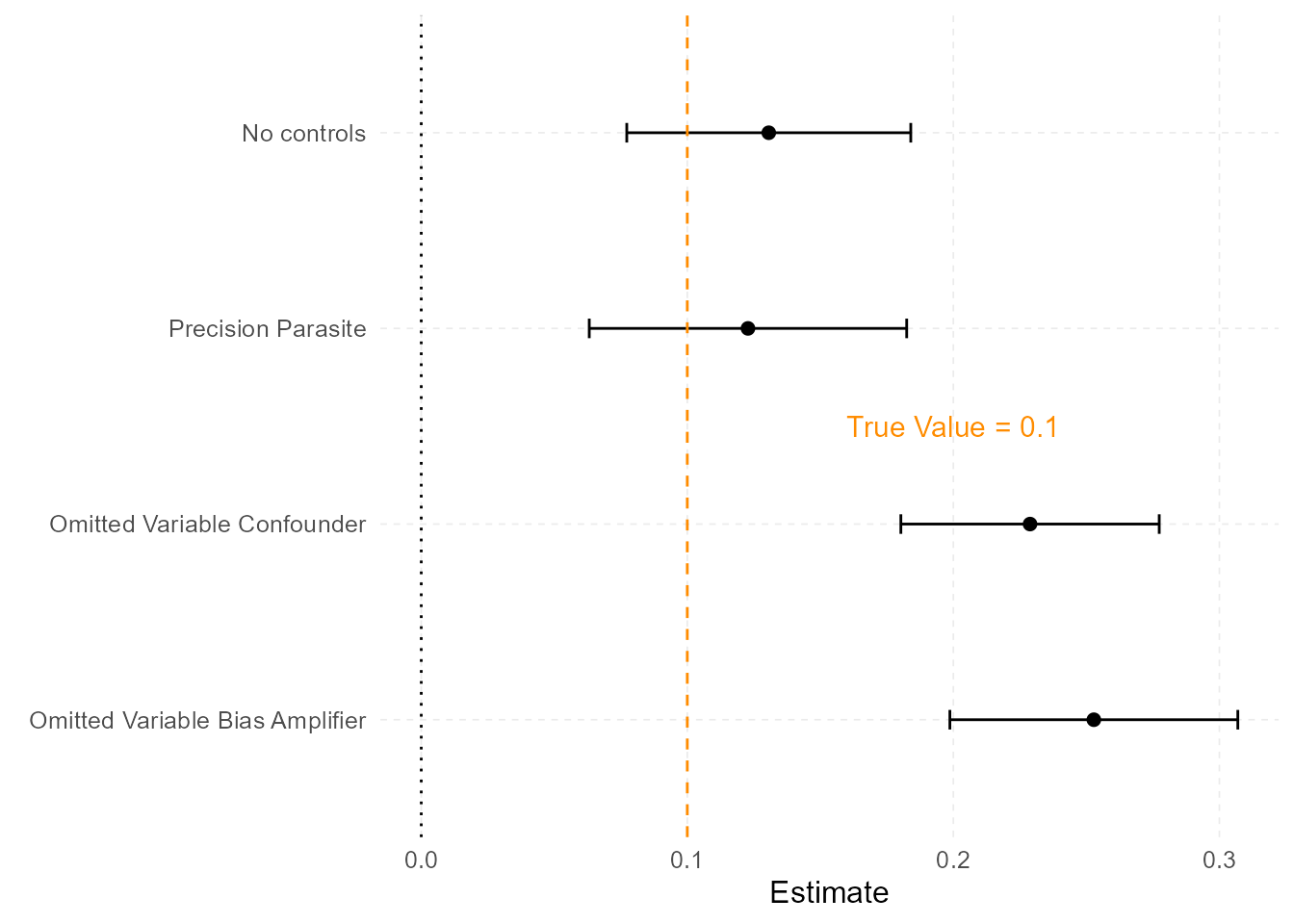
Column 1 of ?tbl-models-parasite shows how our regression captures the effect of \(Education\) on \(log(Income\)) in accordance with the true model. The coefficient on \(Education\) is 0.131 which is close to the true value of \(0.1\). Notice how in Column 2 which still contains no omitted variable, inclusion of the \(Parent Education\) variable in the regression actually increased the uncertainty on the coefficient on \(Education\). The standard error was originally 0.027 but has now increased to 0.03. This is a 10.54 percent increase in the standard error. Also notice that the inclusion of the Precision Parasite did not substantively alter the actual value of the coefficient on \(Education\). This can be seen visually in the top two rows of ?fig-coefplot-parasite where the confidence interval on the coefficient for \(Education\) has increased.
Now we turn to the second estimation results. Here the true model now contains an unobserved variable \(Ability\). In column 3 we can clearly see that omitting the variable \(Ability\) from the regression biases the estimate of the coefficient on \(Education\). In our simulation, we have forced \(Ability\) to exhibit positive covariation with both \(Education\) and \(log(Income)\). This is causing a positive bias on the coefficient on \(Education\) leading to spurious results. Recall the true effect of \(Education\) on \(log(Income)\) is 0.1 in the simulation so this bias is causing a 75.18 percent spurious increase in our estimator of interest.
The real problem now comes in when we also include the Precision Parasite in the regression with the omitted variable \(Ability\). Mathematically, we are now stratifying by \(Parent Education\). The model now looks for variation of \(Education\) within each level of \(Parent Educatino\). Due to there being less variation of \(Education\) after the stratification, the importance of the omitted variable \(Ability\) increases relative to the case without the inclusion of \(Parent Education\). The variable \(Ability\) in the regression now acts as a Bias Amplifier further biasing the coefficient on \(Education\) above and beyond the bias we saw through just the omission of the variable \(Ability\) without stratifying by \(Parent Education\). Again, ?fig-coefplot-parasite shows this visually and it is easy to see the increase in the estimate on \(Education\) deviates even farther from the true value of 0.1 through the inclusion of the Bias Amplifier\(Parent Education\). The value of the coefficient on \(Education\) is 0.253 and now exhibits a 93.54 percent spurious increase compared to the true model value of the coefficient of 0.131.
Exploration of the Precision Parasite and Bias Amplifier in real wage data
We now turn to the wage data-set Wooldridge (2019) in order to see this phenomena in real earnings data. Obviously our “true” model is now quite up for debate, but for illustrative purposes we will have the “true” model contain \(Ability\), \(Experience\), and \(Experience^2\) which clearly have an affect on \(log(Income)\). This time we will first estimate the coefficient on \(Education\) while including \(Ability\)\(Experience\) and \(Experience^2\) in the regression in order to show the Precision Parasite, then we will omit these independent variables from the final two regressions to see how including \(Parent Education\) amplifies the bias on the coefficient of interest.
Table 3.2 shows summary statistics for select variables in the wage data-set.
The following set of linear equations show how we will estimate the effect of \(Education\) on \(log(wage)\). Equation 3.5 and Equation 3.6 will be the “true” model used to show the Precision Parasite. Equation 3.7 and Equation 3.8 will be used to show how the inclusion of \(Parent Education\) acts as an amplifier to the bias affecting the coefficient of interest.
#| label: tbl-wooldridge-regressions#| fig-cap: "OLS regression outputs showing Precision Parasite and Bias Amplifier (wooldridge data)"#| fig-height: 2.5# OLS regression without stratifying by parent educwage_ols_1 <-lm(lwage ~ educ + exper + exper2 + IQ, data = wage_df)# OLS regression controlling for parent educ (Precision Parasite)wage_ols_2 <-lm(lwage ~ educ + fam_educ + exper + exper2 + IQ, data = wage_df)# OLS regression without stratifying by parent educ (with omitted variable)wage_ols_3 <-lm(lwage ~ educ, data = wage_df)# OLS regression with stratifying by parent educ (with omitted variable)wage_ols_4 <-lm(lwage ~ educ + fam_educ, data = wage_df)# Create the regression table using modelsummarywage_models <-list("True Model"= wage_ols_1,"+ Precision Parasite"= wage_ols_2,"OVB"= wage_ols_3,"+ Bias Amplifier"= wage_ols_4 )wage_coef_labels <-c("(Intercept)"="Intercept","educ"="Education","exper"="Experience","exper2"="Experience^2","IQ"="Ability","fam_educ"="Parents' Education")modelsummary(wage_models, coef_map = wage_coef_labels,format_numeric =3, # number of decimal placesstatistic ="std.error", # Show standard errorsstars =FALSE, # Remove significance starsconf_level =0.95, # Confidence interval levelalign ="lcccc", # Align columnsgof_omit ='AIC|BIC|R2 Adj.|RMSE|Std.Errors|R2 Within Adj.|R2 Within|Log.Lik.|F', # Omit statsoutput ="kableExtra",notes ="Note: Estimated coefficients with standard errors in brackets." )
True Model
+ Precision Parasite
OVB
+ Bias Amplifier
Intercept
5.214
5.218
5.973
5.935
(0.133)
(0.149)
(0.081)
(0.093)
Education
0.057
0.051
0.060
0.047
(0.007)
(0.009)
(0.006)
(0.007)
Experience
0.016
0.008
(0.013)
(0.015)
Experience^2
0.000
0.001
(0.001)
(0.001)
Ability
0.006
0.005
(0.001)
(0.001)
Parents' Education
0.019
0.021
(0.006)
(0.006)
Num.Obs.
935
722
935
722
R2
0.162
0.180
0.097
0.113
Note: Estimated coefficients with standard errors in brackets.
Show code
# Function to tidy and extract coefficients and CIsextract_coef_ci <-function(model, model_name) {tidy(model, conf.int =TRUE) |>clean_names() |>mutate(ci =glue("[{round(conf_low, 2)}, {round(conf_high, 2)}]"),model = model_name ) |>select(term, estimate, conf_low, conf_high, model)}# Extract coefficients from different modelswage_coefs_ols_1 <-extract_coef_ci(wage_ols_1, "True Model")wage_coefs_ols_2 <-extract_coef_ci(wage_ols_2, "Precision Parasite")wage_coefs_ols_3 <-extract_coef_ci(wage_ols_3, "Omitted Variable Confounder")wage_coefs_ols_4 <-extract_coef_ci(wage_ols_4, "Omitted Variable Bias Amplifier")# Combine coefficients into one data frameall_coefs_wage <-bind_rows(wage_coefs_ols_1, wage_coefs_ols_2, wage_coefs_ols_3, wage_coefs_ols_4) |>filter(term =="educ")# Reorder the model levels for x-axis orderingall_coefs_wage$model <-factor(all_coefs_wage$model, levels =c("Omitted Variable Bias Amplifier", "Omitted Variable Confounder", "Precision Parasite", "True Model"))#Recalculate the standard error from the confidence intervalsall_coefs_wage$std_error = (all_coefs_wage$conf_high - all_coefs_wage$conf_low) / (2*1.96)
?tbl-wooldridge-regressions shows the regression output for the wage data. Column 1 shows the “true” model which captures the effect of \(Education\) on \(log(wage)\) while controlling for \(Experience\), \(Experience^2\), and \(Ability\). Column 2 shows the “true” model but with the addition of the variable \(Parent Education\). Interestingly, the coefficient \(\beta_1\) on \(Education\) does change by about \(10\) percent with the inclusion of \(Parent Education\) this is probably due to there exisiting other variables or confounds in what we are considering the “true” model for our illustrative purposes. Interestingly, the standard error on the coefficient does increase as expected from a Precision Parasite. The standard error increases by 15.62 percent. The fact that the coefficient on \(Education\) also changes somewhat is probably due to further omitted variable bias that we are failing to capture in the “true” model.
Columns 3 and 4 explore how the omitted variables affecting both \(Education\) and \(log(wage)\) exacerbates the bias on the coefficient of interest. Inclusion of the term \(Parent Education\) caused the coefficient on \(Education\) to display a 21.65 percent change between specifications 3 and 4. Unfortunately the inclusion of the \(Parent Education\) term seems to be biasing the estimated coefficient in the wrong direction. This is probably due to other elemental confounds at play here or it may be an indicator that \(Parent Education\) is in fact through some mechanism not only effecting \(Education\) but also has some direct effect itself on \(log(wage)\). \(Experience\) or \(Ability\) may also be acting as in other confounding ways.
The end.
McElreath, Richard, “Statistical rethinking: A bayesian course with examples in r and STAN,” (Chapman; Hall/CRC, 2020).
Wooldridge, Jeffrey M., “Introductory econometrics: A modern approach,” (Cengage Learning, 2019).
Source Code
# Exploration of Additional Biasing ProblemsThe section is a replication by work of @Mcelreath2020 who uses simulated data to explore how causal effects can be confounded through improper inclusion of control variables in statistical models. Here we will specifically focus on attempting to discern the treatment effect of a variable on an outcome variable but we will include un-observables as well as potential confounders. The author's original video used for this replication can be seen at [Statistical Rethinking video(s)](https://youtu.be/mBEA7PKDmiY?si=vK9oTVePulzZxg6P). We specifically explore the problem of including a **Precision Parasite** and how this actually turns into a **Bias Amplifier** if there are other omitted variables at play in the true model.## Simulation model for the **"Precision Parasite"** and the **"Bias Amplifier"**.```{r}#| label: fig-dags-parasite#| fig-cap: "Some Examples of Bad Controls [@Mcelreath2020]"#| fig-height: 2.5# Load required librarieslibrary("tidyverse")library("modelsummary")library("janitor")library("broom")library("glue")library("kableExtra")library("patchwork")library("ggdag")library("dagitty")# Adapted from @Kurz2023:gg_simple_dag <-function(d) { d %>%ggplot(aes(x = x, y = y, xend = xend, yend = yend)) +geom_dag_point(color ="lightblue", alpha =1/2, size =6.5) +geom_dag_text(color ="gray10") +geom_dag_edges() +theme_dag()}d_parasite <-dagitty("dag { bb=\"0,0,1,1\" X [exposure,pos=\"0.352,0.453\"] Y [outcome,pos=\"0.730,0.450\"] Z [pos=\"0.352,0.201\"] X -> Y Z -> X}")d_bias_amplification <-dagitty(" dag { bb=\"0,0,1,1\" X [exposure,pos=\"0.352,0.453\"] Y [outcome,pos=\"0.730,0.450\"] Z [pos=\"0.352,0.201\"] u [latent,pos=\"0.534,0.201\"] X -> Y Z -> X u -> X u -> Y }")p1 <-gg_simple_dag(d_parasite) +labs(subtitle ="Precision Parasite")p2 <-gg_simple_dag(d_bias_amplification) +labs(subtitle ="Bias Amplification")(p1 | p2) &theme(plot.subtitle =element_text(hjust =0.5))```These models in @fig-dags-parasite illustrate a few important concepts in statistical modelling. In the **"Precision Parasite"** $z$ is not confounding the effect we are looking for of $x$ on $y$. Including $z$ as a control variable seems harmless, however, the problem is that even though the estimated $\beta$ coefficient on $x$ remains unchanged when we include $z$, the precision of $\beta$ becomes worse. A more uncertain estimator could lead us to incorrectly fail to reject the null hypothesis that $\beta = 0$ at some given statistical significance level. The **"Bias Amplification"** situation shown in @fig-dags-parasite is an even more serious problem. Here we also have some un-observable variables that are acting as a *fork* for the effect of $x$ on $y$. We already know from basic econometrics that failing to capture these un-observables biases or confounds the estimate $\beta$ on our variable of interest $x$. Now, however, if we include $z$ as a control variable, the bias actually increases. To illustrate this, we will first produce a **"Precision Parasite"** and **"Bias Amplification"** examples with simulated data, then we will turn to the tried and true education data from @wooldridge2019 and see if we can discover the same outcomes using real data. The following analysis is based on the following set of linear equations.$$\textit{log(Income)} = \alpha_1 + \beta_1 \times \textit{Education} + \epsilon$$ {#eq-inc}$$\textit{Education} = \alpha_2 + \gamma_1 \times \textit{Parent Education} + \epsilon$$ {#eq-educ}- $\alpha_1 = 1.5$: The constant term for *log(Income)*.- $\beta_1 = 0.1$: The effect of *Education* on *log(Income)*.- $\alpha_2 = 6.5$: The constant term for *Education*- $\gamma_1 = 0.55$: The effect of *Parents' Education* on *Individual's Education*.- $\epsilon$: Error terms for unobserved factors influencing *Education* and *log(Income)*.In this first set of equations the true model does not contain "Ability". In other words, in @eq-inc and @eq-educ, there are no variables confounding the model. Only the parent term $Parent Education$ is acting through $Education$ but has no direct influence on $log(Income)$. The following set of linear equations explicitly shows the omitted variable $Ability$.$$\textit{log(Income)} = \alpha_1 + \beta_1 \times \textit{Education} + \beta_2 \times \textit{Ability} + \epsilon$$ {#eq-inc-bias}$$\textit{Education} = \alpha_2 + \gamma_1 \times \textit{Parent Education} + \gamma_2 \times \textit{Ability} + \epsilon$$ {#eq-educ-bias}Where all variables are the same as in the first specification, except:- $\beta_2 = 0.3$: The effect of *Ability* on *log(Income)*. and - $\gamma_2 = 0.6$: The effect of *Ability* on *Individual's Education*.Note the error term is the same in both models. In the second model, the *fork* $Ability$ will be omitted from the regression model for exploration of how inclusion of the **"Precision Parasite"** actually exacerbates the bias introduced from an omitted variable.@tbl-simdata-parasite shows summary statistics for the simulated data-set.```{r}#| label: tbl-simdata-parasite#| tbl-cap: "Synthetic data, simulated based on @eq-inc and @eq-educ"#| tbl-pos: hset.seed(1234)# Number of observationsn <-1000# Simulate an (un)observed confounder (ability) affecting educationability <-rnorm(n)# Simulate an observed value of parent's x (education) affecting x (education)parent_educ <-rnorm(n, mean =12)# Simulate x (education) influenced by z (parent's education)educ <-6.5+0.55* parent_educ +rnorm(n)educ_bias <-6.5+0.55* parent_educ +0.6* ability +rnorm(n)# Simulate income, influenced by x and Zlog_income <-1.5+0.1* educ +rnorm(n)# Simulate omitted variablelog_income_bias <-1.5+0.1* educ_bias +0.3* ability +rnorm(n)# Create the data framesim_data <-data.frame(educ = educ,educ_bias = educ_bias,log_income = log_income,log_income_bias = log_income_bias, parent_educ, ability)# Summary statistics:datasummary(All(sim_data) ~ Mean + SD + Min + Max + N,data = sim_data,output ="kableExtra")```## Estimation resultsEstimation results for the different models are shown in @tbl-models-parasite and a visualization of the coefficients of interest on $Education$ is shown for the four different models in @fig-coefplot-parasite. ```{r}#| label: tbl-models-parasite#| tbl-cap: "Estimation results for Precision Parasite and Bias Amplifier"# OLS regression without stratifying by parent educols_1 <-lm(log_income ~ educ, data = sim_data)# OLS regression controlling for parent educols_2 <-lm(log_income ~ educ + parent_educ, data = sim_data)# OLS regression without stratifying by parent educ (with omitted variable)ols_3 <-lm(log_income_bias ~ educ_bias, data = sim_data)# OLS regression with stratifying by parent educ (with omitted variable)ols_4 <-lm(log_income_bias ~ educ_bias + parent_educ, data = sim_data)# Create the regression table using modelsummarymodels <-list("No controls"= ols_1,"+ Precision Parasite"= ols_2,"Omitted Variable Bias"= ols_3,"+ Bias Amplifier"= ols_4 )coef_labels <-c("(Intercept)"="Intercept","educ"="Education","educ_bias"="Education","parent_educ"="Parents' Education")modelsummary(models, coef_map = coef_labels,format_numeric =3, # number of decimal placesstatistic ="std.error", # Show standard errorsstars =FALSE, # Remove significance starsconf_level =0.95, # Confidence interval levelalign ="lcccc", # Align columnsgof_omit ='AIC|BIC|R2 Adj.|RMSE|Std.Errors|R2 Within Adj.|R2 Within|Log.Lik.|F', # Omit statsoutput ="kableExtra",notes ="Note: Estimated coefficients with standard errors in brackets." ) ``````{r}#| label: fig-coefplot-parasite#| fig-cap: "Estimated coefficients with 95% confidence intervals (simulated data)"#| fig-height: 3# Function to tidy and extract coefficients and CIsextract_coef_ci <-function(model, model_name) {tidy(model, conf.int =TRUE) |>clean_names() |>mutate(ci =glue("[{round(conf_low, 2)}, {round(conf_high, 2)}]"),model = model_name ) |>select(term, estimate, conf_low, conf_high, model)}# Extract coefficients from different modelscoefs_ols_1 <-extract_coef_ci(ols_1, "No controls")coefs_ols_2 <-extract_coef_ci(ols_2, "Precision Parasite")coefs_ols_3 <-extract_coef_ci(ols_3, "Omitted Variable Confounder")coefs_ols_4 <-extract_coef_ci(ols_4, "Omitted Variable Bias Amplifier")# Combine coefficients into one data frameall_coefs_1 <-bind_rows(coefs_ols_1, coefs_ols_2) |>filter(term =="educ")all_coefs_2 <-bind_rows(coefs_ols_3, coefs_ols_4) |>filter(term=="educ_bias")all_coefs <-bind_rows(all_coefs_1, all_coefs_2)# Reorder the model levels for x-axis orderingall_coefs$model <-factor(all_coefs$model, levels =c("Omitted Variable Bias Amplifier", "Omitted Variable Confounder", "Precision Parasite", "No controls"))#Recalculate the standard error from the confidence intervalsall_coefs$std_error = (all_coefs$conf_high - all_coefs$conf_low) / (2*1.96)# Plot coefficients and distinguish models on the x-axisggplot(all_coefs, aes(x = model, y = estimate)) +geom_point(size =2) +geom_errorbar(aes(ymin = conf_low, ymax = conf_high), width =0.1) +labs(y ="Estimate", x =element_blank()) +geom_hline(yintercept =0, linetype ="dotted", color ="black") +# Zero linegeom_hline(yintercept =0.1, linetype ="dashed", color ="darkorange") +# True value linetheme_minimal(base_size =12) +theme(legend.position ="none", # No legend needed since x-axis distinguishes modelspanel.grid.minor =element_blank(),panel.grid.major =element_line(linewidth =0.3, linetype =2) ) +# Add label for the true value horizontal lineannotate("text", x =2.5, y =0.2, label ="True Value = 0.1", color ="darkorange", size =4) +coord_flip()```Column 1 of @tbl-models-parasite shows how our regression captures the effect of $Education$ on $log(Income$) in accordance with the true model. The coefficient on $Education$ is **`r round(all_coefs$estimate[1], 3)`** which is close to the true value of $0.1$. Notice how in Column 2 which still contains no omitted variable, inclusion of the $Parent Education$ variable in the regression actually increased the uncertainty on the coefficient on $Education$. The standard error was originally **`r round(all_coefs$std_error[1], 3)`** but has now increased to **`r round(all_coefs$std_error[2], 3)`**. This is a **`r round(100*(1 - (all_coefs$std_error[1]/all_coefs$std_error[2])), 2)`** percent increase in the standard error. Also notice that the inclusion of the **Precision Parasite** did not substantively alter the actual value of the coefficient on $Education$. This can be seen visually in the top two rows of @fig-coefplot-parasite where the confidence interval on the coefficient for $Education$ has increased. Now we turn to the second estimation results. Here the true model now contains an unobserved variable $Ability$. In column 3 we can clearly see that omitting the variable $Ability$ from the regression biases the estimate of the coefficient on $Education$. In our simulation, we have forced $Ability$ to exhibit positive covariation with both $Education$ and $log(Income)$. This is causing a positive bias on the coefficient on $Education$ leading to spurious results. Recall the true effect of $Education$ on $log(Income)$ is 0.1 in the simulation so this bias is causing a **`r round(((all_coefs$estimate[3] - all_coefs$estimate[1]) / all_coefs$estimate[1])*100, 2)`** percent spurious increase in our estimator of interest. The real problem now comes in when we also include the **Precision Parasite** in the regression with the omitted variable $Ability$. Mathematically, we are now stratifying by $Parent Education$. The model now looks for variation of $Education$ within each level of $Parent Educatino$. Due to there being less variation of $Education$ after the stratification, the importance of the omitted variable $Ability$ increases relative to the case without the inclusion of $Parent Education$. The variable $Ability$ in the regression now acts as a **Bias Amplifier** further biasing the coefficient on $Education$ above and beyond the bias we saw through just the omission of the variable $Ability$ without stratifying by $Parent Education$. Again, @fig-coefplot-parasite shows this visually and it is easy to see the increase in the estimate on $Education$ deviates even farther from the true value of 0.1 through the inclusion of the **Bias Amplifier** $Parent Education$. The value of the coefficient on $Education$ is **`r round(all_coefs$estimate[4], 3)`** and now exhibits a **`r round(100*((all_coefs$estimate[4] - all_coefs$estimate[1]) / all_coefs$estimate[1]), 2)`** percent spurious increase compared to the true model value of the coefficient of **`r round(all_coefs$estimate[1], 3)`**.## Exploration of the **Precision Parasite** and **Bias Amplifier** in real wage dataWe now turn to the **wage** data-set @wooldridge2019 in order to see this phenomena in real earnings data. Obviously our "true" model is now quite up for debate, but for illustrative purposes we will have the "true" model contain $Ability$, $Experience$, and $Experience^2$ which clearly have an affect on $log(Income)$. This time we will first estimate the coefficient on $Education$ while including $Ability$ $Experience$ and $Experience^2$ in the regression in order to show the **Precision Parasite**, then we will omit these independent variables from the final two regressions to see how including $Parent Education$ amplifies the bias on the coefficient of interest.@tbl-wooldridge-statistics shows summary statistics for select variables in the wage data-set.```{r}#| label: tbl-wooldridge-statistics#| fig-cap: "Summary statistics for wage data [@wooldridge2019]"#| fig-height: 2.5# Load required librarieslibrary("wooldridge")# Import the wage datasetwage_df <- wage2wage_df$fam_educ <- (wage_df$meduc + wage_df$feduc) /2wage_df$exper2 <- (wage_df$exper)**2wage_df$tenure2 <- (wage_df$tenure)**2wage_coef_labels <-c("educ"="Education","fam_educ"="Parents' Education","IQ"="Ability","exper"="Experience")selected_wage_data <- wage_df |>select(educ, fam_educ, IQ, exper)# Summary statistics:datasummary(All(selected_wage_data) ~ Mean + SD + Min + Max + N,data = selected_wage_data,coef_map = wage_coef_labels,output ="kableExtra")```The following set of linear equations show how we will estimate the effect of $Education$ on $log(wage)$. @eq-wage-true and @eq-wage-parasite will be the "true" model used to show the **Precision Parasite**. @eq-wage-bias and @eq-wage-bias-amplifier will be used to show how the inclusion of $Parent Education$ acts as an amplifier to the bias affecting the coefficient of interest.$$\begin{split}\textit{log(wage)} = \alpha_1 + \beta_1 \times \textit{Education} + \beta_2 \times \textit{Experience} + \\\beta_3 \times Experience^2+ \beta_4 \times \textit{Ability} + \epsilon\end{split}$$ {#eq-wage-true}$$\begin{split}\textit{log(wage)} = \alpha_1 + \beta_1 \times \textit{Education} + \beta_2 \times \textit{Experience} + \beta_3 \times Experience^2+ \\\beta_4 \times \textit{Ability} + \beta_5 \times \textit{Parent Education} +\epsilon\end{split}$$ {#eq-wage-parasite}$$\textit{log(wage)} = \alpha_1 + \gamma_1 \times \textit{Education} + \epsilon$$ {#eq-wage-bias}$$\textit{log(wage)} = \alpha_1 + \gamma_1 \times \textit{Education} + \gamma_2 \times \textit{Parent Education} +\epsilon$$ {#eq-wage-bias-amplifier}```{r}#| label: tbl-wooldridge-regressions#| fig-cap: "OLS regression outputs showing Precision Parasite and Bias Amplifier (wooldridge data)"#| fig-height: 2.5# OLS regression without stratifying by parent educwage_ols_1 <-lm(lwage ~ educ + exper + exper2 + IQ, data = wage_df)# OLS regression controlling for parent educ (Precision Parasite)wage_ols_2 <-lm(lwage ~ educ + fam_educ + exper + exper2 + IQ, data = wage_df)# OLS regression without stratifying by parent educ (with omitted variable)wage_ols_3 <-lm(lwage ~ educ, data = wage_df)# OLS regression with stratifying by parent educ (with omitted variable)wage_ols_4 <-lm(lwage ~ educ + fam_educ, data = wage_df)# Create the regression table using modelsummarywage_models <-list("True Model"= wage_ols_1,"+ Precision Parasite"= wage_ols_2,"OVB"= wage_ols_3,"+ Bias Amplifier"= wage_ols_4 )wage_coef_labels <-c("(Intercept)"="Intercept","educ"="Education","exper"="Experience","exper2"="Experience^2","IQ"="Ability","fam_educ"="Parents' Education")modelsummary(wage_models, coef_map = wage_coef_labels,format_numeric =3, # number of decimal placesstatistic ="std.error", # Show standard errorsstars =FALSE, # Remove significance starsconf_level =0.95, # Confidence interval levelalign ="lcccc", # Align columnsgof_omit ='AIC|BIC|R2 Adj.|RMSE|Std.Errors|R2 Within Adj.|R2 Within|Log.Lik.|F', # Omit statsoutput ="kableExtra",notes ="Note: Estimated coefficients with standard errors in brackets." ) # Function to tidy and extract coefficients and CIsextract_coef_ci <-function(model, model_name) {tidy(model, conf.int =TRUE) |>clean_names() |>mutate(ci =glue("[{round(conf_low, 2)}, {round(conf_high, 2)}]"),model = model_name ) |>select(term, estimate, conf_low, conf_high, model)}# Extract coefficients from different modelswage_coefs_ols_1 <-extract_coef_ci(wage_ols_1, "True Model")wage_coefs_ols_2 <-extract_coef_ci(wage_ols_2, "Precision Parasite")wage_coefs_ols_3 <-extract_coef_ci(wage_ols_3, "Omitted Variable Confounder")wage_coefs_ols_4 <-extract_coef_ci(wage_ols_4, "Omitted Variable Bias Amplifier")# Combine coefficients into one data frameall_coefs_wage <-bind_rows(wage_coefs_ols_1, wage_coefs_ols_2, wage_coefs_ols_3, wage_coefs_ols_4) |>filter(term =="educ")# Reorder the model levels for x-axis orderingall_coefs_wage$model <-factor(all_coefs_wage$model, levels =c("Omitted Variable Bias Amplifier", "Omitted Variable Confounder", "Precision Parasite", "True Model"))#Recalculate the standard error from the confidence intervalsall_coefs_wage$std_error = (all_coefs_wage$conf_high - all_coefs_wage$conf_low) / (2*1.96)```@tbl-wooldridge-regressions shows the regression output for the wage data. Column 1 shows the "true" model which captures the effect of $Education$ on $log(wage)$ while controlling for $Experience$, $Experience^2$, and $Ability$. Column 2 shows the "true" model but with the addition of the variable $Parent Education$. Interestingly, the coefficient $\beta_1$ on $Education$ does change by about $10$ percent with the inclusion of $Parent Education$ this is probably due to there exisiting other variables or confounds in what we are considering the "true" model for our illustrative purposes. Interestingly, the standard error on the coefficient does increase as expected from a **Precision Parasite**. The standard error increases by **`r round(100*((all_coefs_wage$std_error[2]-all_coefs_wage$std_error[1])/all_coefs_wage$std_error[1]), 2)`** percent. The fact that the coefficient on $Education$ also changes somewhat is probably due to further omitted variable bias that we are failing to capture in the "true" model.Columns 3 and 4 explore how the omitted variables affecting both $Education$ and $log(wage)$ exacerbates the bias on the coefficient of interest. Inclusion of the term $Parent Education$ caused the coefficient on $Education$ to display a **`r round(100*((all_coefs_wage$estimate[3]-all_coefs_wage$estimate[4])/all_coefs_wage$estimate[3]), 2)`** percent change between specifications 3 and 4. Unfortunately the inclusion of the $Parent Education$ term seems to be biasing the estimated coefficient in the wrong direction. This is probably due to other elemental confounds at play here or it may be an indicator that $Parent Education$ is in fact through some mechanism not only effecting $Education$ but also has some direct effect itself on $log(wage)$. $Experience$ or $Ability$ may also be acting as in other confounding ways.The end.