A key challenge in causal inference is dealing with endogeneity, where variables affect each other and we need to address reverse causality or omitted variable bias.
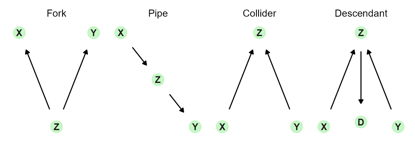
The following exercise illustrates two of the “elemental confounds”: The fork and the collider.1
Figure 2.1: The four elemental confounds (Kurz 2023)
Simulation: confounding and collider bias
Here, we focus on a confounder \(z\) that affects both the dependent variable \(y\) and an independent variable \(x\), plus a collider \(w\) that is affected by both. To better understand the problem, we simulate data and test alternative models.
We will simulate data for 1000 hypothetical observations, based on the following structure:
\[
z \sim \mathcal{N}(\mu,\sigma^2)
\tag{2.1}\]
\[
x = \alpha_1 + \alpha_2\ z + \epsilon_1
\tag{2.2}\]
\[
y = \beta_1\ x + \beta_2\ z + \epsilon_2
\tag{2.3}\]
The confounder \(z\) is normally distributed with mean \(\mu\) and variance \(\sigma^2\); \(x\) depends on a constant term and \(z\) (Equation 2.2), \(y\) is affected by both \(x\) and \(z\) (Equation 2.3), and \(w\) is determined based on \(x\) and \(y\) (Equation 2.4).
For the simulation, we set the following parameter values:
\(\mu = 50,\ \sigma=5\): \(z\) is normally distributed with mean 50 and variance 25.
\(\alpha_1 = 2\): The constant term for x, \(\alpha_2 = 0.3\): The effect of z on x.
\(\beta_1 = -0.3\), \(\beta_2 = -0.5\): The effect of x and z on y
\(\gamma_1 = -0.3\), \(\gamma_2 = -0.5\): The effect of x and y on w.
\(\epsilon_1, \epsilon_2\) and \(\epsilon_3\): Error terms, following a normal distribution with mean zero
Show code
# Load required librarieslibrary("tidyverse")library("modelsummary")library("broom")library("glue")library("kableExtra")# Set random seedset.seed(41)# Number of observationsn <-1000# Simulate an (un)observed confounder affecting both x and conflictz <-rnorm(n, mean =50, sd =5)# Simulate x influenced by political Zx <-2+0.3* z +rnorm(n)# Simulate conflict, influenced by x and Zy <--0.5* z -0.3* x +rnorm(n)# Simulate colliderw =-0.5* x +0.6* y +rnorm(n)# Create the data framesim_data <-data.frame(z = z,w = w,x = x,y = y)# Summary statistics:datasummary(All(sim_data) ~ Mean + SD + Min + Max + N,data = sim_data,output ="kableExtra")
Table 2.1: Synthetic data, summary statistics
Mean
SD
Min
Max
N
z
50.02
4.98
33.71
66.63
1000
w
−26.54
2.84
−34.79
−16.09
1000
x
16.98
1.83
11.46
21.85
1000
y
−30.08
3.16
−40.21
−19.00
1000
Estimation results
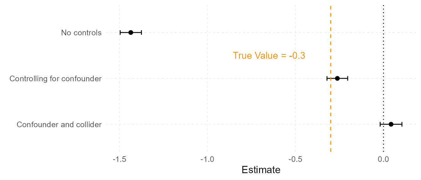
Our main coefficient of interest is \(\beta_1\), the effect of \(x\) on \(y\), which we simulated as \(-0.3\). We estimate three linear models with \(y\) as the dependent variable: (1) \(x\) without control variables, (2) controlling for \(z\), and (3) controlling for both \(z\) and \(w\).
Estimation results for the different models are shown in Table 2.2 and Figure 2.2.
Show code
# OLS regression without controlsols_1 <-lm(y ~ x, data = sim_data)# OLS regression controlling for the confounderols_2 <-lm(y ~ x + z, data = sim_data)# OLS regression controlling for the both confounder and colliderols_3 <-lm(y ~ x + z + w, data = sim_data)# Create the regression table using modelsummarymodels <-list("No controls"= ols_1,"+ Confounder"= ols_2,"+ Collider"= ols_3 )coef_labels <-c("(Intercept)"="Intercept","x"="x","z"="z","w"="w")m =modelsummary(models, coef_map = coef_labels,format_numeric =3, # number of decimal placesstatistic ="conf.int", # Show confidence intervals instead of standard errorsstars =FALSE, # Remove significance starsconf_level =0.95, # Confidence interval levelalign ="lccc", # Align columnsgof_omit ='AIC|BIC|R2 Adj.|RMSE|Std.Errors|R2 Within Adj.|R2 Within|Log.Lik.|F', # Omit statsoutput ="kableExtra",notes ="Note: Estimated coefficients with 95% confidence intervals in brackets." ) m
Table 2.2: Estimation results
No controls
+ Confounder
+ Collider
Intercept
−5.690
0.512
0.522
[−6.719, −4.661]
[−0.113, 1.137]
[−0.025, 1.068]
x
−1.436
−0.262
0.043
[−1.496, −1.376]
[−0.321, −0.203]
[−0.019, 0.105]
z
−0.523
−0.398
[−0.544, −0.501]
[−0.421, −0.374]
w
0.431
[0.382, 0.479]
Num.Obs.
1000
1000
1000
R2
0.687
0.904
0.927
Note: Estimated coefficients with 95% confidence intervals in brackets.
Show code
# Function to tidy and extract coefficients and CIsextract_coef_ci <-function(model, model_name) {tidy(model, conf.int =TRUE) |>clean_names() |>mutate(ci =glue("[{round(conf_low, 2)}, {round(conf_high, 2)}]"),model = model_name ) |>select(term, estimate, conf_low, conf_high, model)}# Extract coefficients from different modelscoefs_ols_1 <-extract_coef_ci(ols_1, "No controls")coefs_ols_2 <-extract_coef_ci(ols_2, "Controlling for confounder")coefs_ols_3 <-extract_coef_ci(ols_3, "Confounder and collider")# Combine coefficients into one data frameall_coefs <-bind_rows(coefs_ols_1, coefs_ols_2, coefs_ols_3) |>filter(term =="x")# Reorder the model levels for x-axis orderingall_coefs$model <-factor(all_coefs$model, levels =c("Confounder and collider", "Controlling for confounder", "No controls"))# Plot coefficients and distinguish models on the x-axisggplot(all_coefs, aes(x = model, y = estimate)) +geom_point(size =2) +geom_errorbar(aes(ymin = conf_low, ymax = conf_high), width =0.1) +labs(y ="Estimate", x =element_blank()) +geom_hline(yintercept =0, linetype ="dotted", color ="black") +# Zero linegeom_hline(yintercept =-0.3, linetype ="dashed", color ="darkorange") +# True value linetheme_minimal(base_size =12) +theme(legend.position ="none", # No legend needed since x-axis distinguishes modelspanel.grid.minor =element_blank(),panel.grid.major =element_line(linewidth =0.3, linetype =2) ) +# Add label for the true value horizontal lineannotate("text", x =2.5, y =-0.65, label ="True Value = -0.3", color ="darkorange", size =4) +coord_flip()
Figure 2.2: Estimated coefficients with 95% confidence intervals
# Confounding and collider biasA key challenge in causal inference is dealing with **endogeneity**, where variables affect each other and we need to address **reverse causality** or **omitted variable bias**.The following exercise illustrates two of the **"elemental confounds"**: The *fork* and the *collider*.^[Check @Mcelreath2020 and the [Statistical Rethinking video(s)](https://youtu.be/mBEA7PKDmiY?si=vK9oTVePulzZxg6P) for a great introduction.]```{r}#| label: fig-dags#| fig-cap: "The four elemental confounds [@Kurz2023]"#| fig-height: 2.5# Load required librarieslibrary("tidyverse")library("modelsummary")library("janitor")library("broom")library("glue")library("kableExtra")library("patchwork")library("ggdag")# Adapted from @Kurz2023:gg_simple_dag <-function(d) { d %>%ggplot(aes(x = x, y = y, xend = xend, yend = yend)) +geom_dag_point(color ="lightgreen", alpha =1/2, size =6.5) +geom_dag_text(color ="gray10") +geom_dag_edges() +theme_dag()}d1 <-dagify(X ~ Z, Y ~ Z,coords =tibble(name =c("X", "Y", "Z"),x =c(1, 3, 2),y =c(2, 2, 1)))d2 <-dagify(Z ~ X, Y ~ Z,coords =tibble(name =c("X", "Y", "Z"),x =c(1, 3, 2),y =c(2, 1, 1.5)))d3 <-dagify(Z ~ X + Y,coords =tibble(name =c("X", "Y", "Z"),x =c(1, 3, 2),y =c(1, 1, 2)))d4 <-dagify(Z ~ X + Y, D ~ Z,coords =tibble(name =c("X", "Y", "Z", "D"),x =c(1, 3, 2, 2),y =c(1, 1, 2, 1.05)))p1 <-gg_simple_dag(d1) +labs(subtitle ="Fork")p2 <-gg_simple_dag(d2) +labs(subtitle ="Pipe")p3 <-gg_simple_dag(d3) +labs(subtitle ="Collider")p4 <-gg_simple_dag(d4) +labs(subtitle ="Descendant")(p1 | p2 | p3 | p4) &theme(plot.subtitle =element_text(hjust =0.5))```## Simulation: confounding and collider biasHere, we focus on a confounder $z$ that affects both the dependent variable $y$ and an independent variable $x$, plus a collider $w$ that is affected by both. To better understand the problem, we simulate data and test alternative models.We will simulate data for 1000 hypothetical observations, based on the following structure: $$z \sim \mathcal{N}(\mu,\sigma^2)$$ {#eq-z}$$x = \alpha_1 + \alpha_2\ z + \epsilon_1$$ {#eq-x}$$y = \beta_1\ x + \beta_2\ z + \epsilon_2$$ {#eq-y}$$w = \gamma_1\ \textit{x} + \gamma_2\ \textit{y} + \epsilon_2$$ {#eq-w}The confounder $z$ is normally distributed with mean $\mu$ and variance $\sigma^2$; $x$ depends on a constant term and $z$ (@eq-x), $y$ is affected by both $x$ and $z$ (@eq-y), and $w$ is determined based on $x$ and $y$ (@eq-w).For the simulation, we set the following parameter values:- $\mu = 50,\ \sigma=5$: $z$ is normally distributed with mean 50 and variance 25.- $\alpha_1 = 2$: The constant term for *x*, $\alpha_2 = 0.3$: The effect of *z* on *x*.- $\beta_1 = -0.3$, $\beta_2 = -0.5$: The effect of *x* and *z* on *y*- $\gamma_1 = -0.3$, $\gamma_2 = -0.5$: The effect of *x* and *y* on *w*.- $\epsilon_1, \epsilon_2$ and $\epsilon_3$: Error terms, following a normal distribution with mean zero```{r}#| label: tbl-simdata-1#| tbl-cap: "Synthetic data, summary statistics"# Load required librarieslibrary("tidyverse")library("modelsummary")library("broom")library("glue")library("kableExtra")# Set random seedset.seed(41)# Number of observationsn <-1000# Simulate an (un)observed confounder affecting both x and conflictz <-rnorm(n, mean =50, sd =5)# Simulate x influenced by political Zx <-2+0.3* z +rnorm(n)# Simulate conflict, influenced by x and Zy <--0.5* z -0.3* x +rnorm(n)# Simulate colliderw =-0.5* x +0.6* y +rnorm(n)# Create the data framesim_data <-data.frame(z = z,w = w,x = x,y = y)# Summary statistics:datasummary(All(sim_data) ~ Mean + SD + Min + Max + N,data = sim_data,output ="kableExtra")```## Estimation resultsOur main coefficient of interest is $\beta_1$, the effect of $x$ on $y$, which we simulated as $-0.3$. We estimate three linear models with $y$ as the dependent variable: (1) $x$ without control variables, (2) controlling for $z$, and (3) controlling for both $z$ and $w$.Estimation results for the different models are shown in @tbl-models-1 and @fig-coefplot. ```{r}#| label: tbl-models-1#| tbl-cap: "Estimation results"# OLS regression without controlsols_1 <-lm(y ~ x, data = sim_data)# OLS regression controlling for the confounderols_2 <-lm(y ~ x + z, data = sim_data)# OLS regression controlling for the both confounder and colliderols_3 <-lm(y ~ x + z + w, data = sim_data)# Create the regression table using modelsummarymodels <-list("No controls"= ols_1,"+ Confounder"= ols_2,"+ Collider"= ols_3 )coef_labels <-c("(Intercept)"="Intercept","x"="x","z"="z","w"="w")m =modelsummary(models, coef_map = coef_labels,format_numeric =3, # number of decimal placesstatistic ="conf.int", # Show confidence intervals instead of standard errorsstars =FALSE, # Remove significance starsconf_level =0.95, # Confidence interval levelalign ="lccc", # Align columnsgof_omit ='AIC|BIC|R2 Adj.|RMSE|Std.Errors|R2 Within Adj.|R2 Within|Log.Lik.|F', # Omit statsoutput ="kableExtra",notes ="Note: Estimated coefficients with 95% confidence intervals in brackets." ) m ``````{r}#| label: fig-coefplot#| fig-cap: "Estimated coefficients with 95% confidence intervals"#| fig-height: 3# Function to tidy and extract coefficients and CIsextract_coef_ci <-function(model, model_name) {tidy(model, conf.int =TRUE) |>clean_names() |>mutate(ci =glue("[{round(conf_low, 2)}, {round(conf_high, 2)}]"),model = model_name ) |>select(term, estimate, conf_low, conf_high, model)}# Extract coefficients from different modelscoefs_ols_1 <-extract_coef_ci(ols_1, "No controls")coefs_ols_2 <-extract_coef_ci(ols_2, "Controlling for confounder")coefs_ols_3 <-extract_coef_ci(ols_3, "Confounder and collider")# Combine coefficients into one data frameall_coefs <-bind_rows(coefs_ols_1, coefs_ols_2, coefs_ols_3) |>filter(term =="x")# Reorder the model levels for x-axis orderingall_coefs$model <-factor(all_coefs$model, levels =c("Confounder and collider", "Controlling for confounder", "No controls"))# Plot coefficients and distinguish models on the x-axisggplot(all_coefs, aes(x = model, y = estimate)) +geom_point(size =2) +geom_errorbar(aes(ymin = conf_low, ymax = conf_high), width =0.1) +labs(y ="Estimate", x =element_blank()) +geom_hline(yintercept =0, linetype ="dotted", color ="black") +# Zero linegeom_hline(yintercept =-0.3, linetype ="dashed", color ="darkorange") +# True value linetheme_minimal(base_size =12) +theme(legend.position ="none", # No legend needed since x-axis distinguishes modelspanel.grid.minor =element_blank(),panel.grid.major =element_line(linewidth =0.3, linetype =2) ) +# Add label for the true value horizontal lineannotate("text", x =2.5, y =-0.65, label ="True Value = -0.3", color ="darkorange", size =4) +coord_flip()```